AI is definitely the hottest topic in computer science right now (perhaps next to Blockchain of course) so I thought I’d give a brief tutorial on how this works. You may have heard that massive GPUs crunch a bunch of “stuff” to make predictions, and if you paid even more attention you know that the secret sauce is called a neural network. So let’s look at building just a single “neuron” for demonstrating the basic concept behind neural networks and hopefully that will demystify all this AI stuff.
Building Machine Learning Models from Scratch
- Machine Learning in a Nutshell: Computers can learn to find patterns in data without needing every step spelled out. Imagine teaching a computer to tell the difference between photos of cats and dogs!
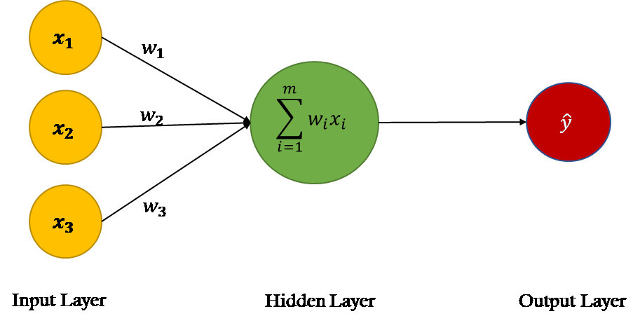
- The Power of a Single Neuron: We’ll start with the building block of many large, complex models. A single neuron is like a tiny calculator that takes in data and produces a prediction.
- Python to the Rescue: Python gives us the tools to write our own instructions to train these little neurons, just like building a muscle with exercise!
- Step by Step: We’ll start by focusing on the core math behind it all. Don’t worry, no fancy libraries needed for now – this makes understanding the basics easier.
Machine Learning with Simple Math
Imagine you have a machine learning model that’s like a simple calculator. It takes in data points (xi) and tries to predict a real value (yi) for each one.
In this example, we’re building the model from scratch using Python functions. We can write the code to do two key things:
- Forward Calculation: This is like the calculator part. It takes a data point (xi) as input and uses some math (f(xi)) to come up with a predicted value (yi).
- Weight Adjustment: The model isn’t perfect at first, so we need a way to adjust it. Here’s where the fun part comes in! We can calculate how wrong the predictions are (gradient) and use that information to slightly change the model’s internal numbers (weights or coefficients). This is like fine-tuning the calculator.
By repeatedly doing these calculations (forward pass and weight update) with many data points, the model gradually learns to make better predictions. This is a technique called gradient descent.
Key Points:
- We’re building a simple model to understand the core concepts.
- We write Python functions to do the calculations ourselves (no fancy libraries yet).
- The model learns by adjusting its internal numbers based on how wrong its predictions are.
Training: Teaching Our Model to See
Think of your regression model like a student who needs practice before a big test. Training is the study session!
Cost Function: The Study Guide. This tells us how far off our model’s predictions are currently (like a practice test highlighting mistakes).
Gradient Descent: The Smart Tutor. It guides the model to make better guesses. It looks at the cost function and says, “change your weights a tiny bit this way to do better next time.”
Loops and Epochs – Practice Makes Perfect
- Training Loops: Each time the model goes through the entire dataset and has its weights adjusted, we call that a training loop (or epoch). It’s like doing multiple practice problems.
- Iterations: Within each loop, the model looks at smaller chunks of data, updating its weights each time. These are iterations, like working through each problem within a practice test.
The Goal: Finding the A+ Solution
The gradient descent wants the model to get the lowest score possible on the cost function ‘test’. This means the smallest difference between its predictions and the real answers.
Key Takeaways:
- Training is essential for a model to make accurate predictions.
- Gradient descent is a clever method to guide the model towards better ‘answers’.
- Think of training loops and iterations as the model’s structured practice session.
The Hiker Analogy:
Imagine our regression model is a blindfolded hiker trying to find the lowest point in a valley. They don’t start with a map! Cost Function: This is like the hiker feeling around their feet to figure out the slope of the ground. A steep slope means they’re far from the bottom (high cost). Gradient Descent: This is the hiker’s technique. Feel the slope, take a small step in the direction that goes downhill the fastest (that’s the gradient telling them what to do). Training Loops (Epochs): Each full trip the hiker takes down the valley and back up the other side is like one training loop. They get a better sense of the overall terrain. Iterations: Every individual step the hiker takes is an iteration. Each step adjusts their understanding of where the valley floor is.
The Goal: Finding the Valley Floor
The hiker (i.e., the model) wants to find the absolute lowest point in the valley. This is like getting the lowest possible ‘score’ on the cost function, meaning the most accurate predictions possible.


Social Profiles